Using Matrix To Solve System Of Equations
listenit
Mar 26, 2025 · 6 min read
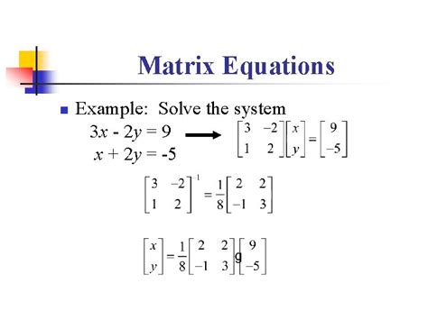
Table of Contents
Using Matrices to Solve Systems of Equations: A Comprehensive Guide
Solving systems of equations is a fundamental task in various fields, from engineering and physics to economics and computer science. While substitution and elimination methods work well for small systems, they become cumbersome and inefficient for larger ones. This is where matrices step in, offering a powerful and elegant solution. This comprehensive guide will explore how matrices can be used to solve systems of equations, covering various methods and their applications.
What are Matrices and Why Use Them?
A matrix is a rectangular array of numbers, symbols, or expressions, arranged in rows and columns. In the context of solving systems of equations, we represent the coefficients of the variables and the constants as a matrix. This representation allows us to use powerful matrix operations to solve the system efficiently.
Using matrices offers several advantages:
- Efficiency: Matrix methods are significantly more efficient for large systems of equations compared to traditional methods.
- Clarity: Representing the system as a matrix provides a clear and concise way to visualize the problem.
- Generalizability: Matrix methods can be easily adapted to solve systems with any number of equations and variables.
- Computational Power: Matrix operations are readily implemented in software packages like MATLAB, Python (with NumPy), and others, allowing for quick solutions to even very large systems.
Representing Systems of Equations with Matrices
Let's consider a system of linear equations:
a₁₁x₁ + a₁₂x₂ + ... + a₁nxₙ = b₁
a₂₁x₁ + a₂₂x₂ + ... + a₂nxₙ = b₂
...
am₁x₁ + am₂x₂ + ... + amnxₙ = bm
This system can be represented using three matrices:
- Coefficient Matrix (A): This matrix contains the coefficients of the variables:
A =  [[a₁₁, a₁₂, ..., a₁ₙ],
      [a₂₁, a₂₂, ..., a₂ₙ],
      [..., ..., ..., ...],
      [am₁, am₂, ..., amₙ]]
- Variable Matrix (X): This matrix contains the variables:
X = [[x₁],
     [x₂],
     [...],
     [xₙ]]
- Constant Matrix (B): This matrix contains the constants on the right-hand side of the equations:
B = [[b₁],
     [b₂],
     [...],
     [bm]]
The system of equations can now be concisely represented as a single matrix equation:
AX = B
Methods for Solving Systems of Equations Using Matrices
Several methods exist for solving the matrix equation AX = B. We will explore two of the most common:
1. Gaussian Elimination (Row Reduction)
Gaussian elimination is a systematic method for transforming the augmented matrix [A|B] (obtained by concatenating A and B) into row echelon form or reduced row echelon form. This process involves elementary row operations:
- Swapping two rows: Interchanging the positions of two rows.
- Multiplying a row by a non-zero scalar: Multiplying all entries in a row by the same non-zero constant.
- Adding a multiple of one row to another row: Adding a multiple of one row to another row.
By applying these operations, we aim to obtain a triangular matrix (row echelon form) or a diagonal matrix (reduced row echelon form). From this form, the solution can be easily obtained through back-substitution.
Example:
Let's solve the following system using Gaussian elimination:
x + 2y = 5
2x - y = 1
The augmented matrix is:
[1  2 | 5]
[2 -1 | 1]
- Subtract 2 times the first row from the second row:
[1  2 | 5]
[0 -5 |-9]
- Divide the second row by -5:
[1  2 | 5]
[0  1 | 9/5]
- Subtract 2 times the second row from the first row:
[1  0 | 7/5]
[0  1 | 9/5]
The solution is x = 7/5 and y = 9/5.
2. Inverse Matrix Method
If the coefficient matrix A is invertible (i.e., its determinant is non-zero), we can find its inverse, denoted as A⁻¹. Multiplying both sides of the equation AX = B by A⁻¹ gives:
A⁻¹AX = A⁻¹B
Since A⁻¹A is the identity matrix (I), we have:
IX = A⁻¹B
Therefore, the solution is simply:
X = A⁻¹B
Finding the inverse of a matrix can be done using various methods, including the adjoint method or through row reduction. However, for larger matrices, computational methods are usually preferred due to their efficiency.
Example:
Consider the same system of equations as before:
x + 2y = 5
2x - y = 1
The coefficient matrix A is:
A = [[1, 2],
     [2, -1]]
The determinant of A is (1)(-1) - (2)(2) = -5. Since the determinant is non-zero, the inverse exists. The inverse of A can be calculated (using methods beyond the scope of this simplified explanation) to be:
A⁻¹ = [-1/5, -2/5]
       [-2/5,  1/5]
Then,
X = A⁻¹B = [-1/5, -2/5]  [5]   =  [7/5]
             [-2/5,  1/5]  [1]   =  [9/5]
This gives the same solution as before: x = 7/5 and y = 9/5.
Choosing the Right Method
The choice between Gaussian elimination and the inverse matrix method depends on the specific problem:
-
Gaussian elimination: Generally more efficient for larger systems, particularly when the matrix is not square or not invertible. It's also less computationally demanding than finding the inverse.
-
Inverse matrix method: Elegant and concise, especially for smaller systems. Useful when the inverse matrix is needed for other calculations. However, it's computationally expensive for large matrices and requires the matrix to be invertible.
Handling Singular Matrices (Non-Invertible Matrices)
If the determinant of the coefficient matrix A is zero, the matrix is singular (non-invertible). This means the system of equations either has no solution (inconsistent system) or infinitely many solutions (dependent system). Gaussian elimination is the best method to handle these cases, as it will reveal the nature of the solution – whether there are no solutions or infinitely many. The process will result in a row of zeros in the augmented matrix indicating the system is dependent (infinite solutions) or a row of zeros with a non-zero constant, indicating the system is inconsistent (no solutions).
Applications of Matrix Methods in Solving Systems of Equations
Matrix methods are widely applied in various fields:
- Engineering: Solving complex structural analysis problems, circuit analysis, and control systems.
- Physics: Solving systems of differential equations, describing particle motion, and analyzing electromagnetic fields.
- Economics: Modeling economic systems, analyzing market equilibrium, and optimizing resource allocation.
- Computer Graphics: Transforming and manipulating 3D objects, calculating lighting effects, and creating realistic animations.
- Machine Learning: Solving linear regression problems, finding optimal parameters in neural networks, and performing dimensionality reduction.
Conclusion
Matrices provide a powerful and efficient tool for solving systems of equations, especially when dealing with large or complex systems. Understanding the different methods – Gaussian elimination and the inverse matrix method – allows you to choose the most appropriate approach based on the specific problem and its characteristics. The ability to represent and manipulate systems of equations using matrices is a fundamental skill in various scientific and engineering disciplines. Mastering these techniques opens up a world of possibilities for tackling complex problems with elegance and efficiency. Remember to always consider the potential for singular matrices and apply the appropriate strategies when encountering such scenarios.
Latest Posts
Latest Posts
-
Standard Enthalpy Of Formation Of Ethanol
Mar 29, 2025
-
Do Parallelograms Have 4 Right Angles
Mar 29, 2025
-
Least Common Multiple Of 10 And 8
Mar 29, 2025
-
Name 3 Ways To Dissolve Something Faster
Mar 29, 2025
-
Charged Language In I Have A Dream
Mar 29, 2025
Related Post
Thank you for visiting our website which covers about Using Matrix To Solve System Of Equations . We hope the information provided has been useful to you. Feel free to contact us if you have any questions or need further assistance. See you next time and don't miss to bookmark.
